If a chimney is the right height, the wind whistles. If a telephone wire is the right thickness, it hums. If a car drives past at the right speed, the antenna shakes. All three are doing the same thing — shedding a Kármán vortex street, pairs of counter-rotating swirls peeling alternately off the back of the obstacle. The rhythm of that shedding sets a frequency, and if some natural mode of the structure happens to live in the same range, the vortex street feeds it.
This post is about what happens when you turn the problem around: not the cylinder being moved by the flow, but the cylinder being forced to move, and what its wake decides to do in response.
1. The wake that’s everywhere
Pick a circular cylinder in a uniform flow at a modest speed. The flow has to go around it; what’s left behind is a wake. Below a critical Reynolds number — roughly $\text{Re} \le 100$ — the wake settles into the same pattern every time: a regular zigzag of vortices, alternating clockwise above and counter-clockwise below. That’s the 2S pattern: two single vortices shed per period. Sometimes called Kármán shedding, after Theodore von Kármán, who first analysed its stability in 1911.
The pattern is symmetric. Top mirrors bottom under reflection plus a half-period time shift. Nothing in the equations of motion prefers one side: the free stream is uniform, the cylinder is round, the whole problem has a left–right symmetry that the solution respects.
2. A cylinder in a steady flow
For context, the Reynolds number is the dimensionless ratio that decides whether viscous or inertial forces dominate:
$$ \text{Re} = \frac{U_\infty D}{\nu} $$
where $U_\infty$ is the free-stream speed, $D$ is the cylinder diameter, and $\nu$ is the kinematic viscosity. Below $\text{Re} \approx 47$ the wake is steady — the flow recirculates symmetrically behind the cylinder and goes nowhere. Above that, the recirculation loses stability: a vortex peels off, then another, and shedding begins. Up to $\text{Re} \approx 200$ the shedding stays two-dimensional and laminar, which is the regime this thesis lives in. The flow can be simulated faithfully in a 2D plane without missing real physics.
The Kármán shedding has its own natural frequency. For a fixed cylinder at $\text{Re} = 100$, the shedding frequency $f_s$ obeys $\text{St} = f_s D / U_\infty \approx 0.165$, where $\text{St}$ is the Strouhal number. That number is the rhythm the wake wants to be in.
3. Now wiggle it
Force the cylinder to oscillate vertically:
$$ y_{\text{cyl}}(t) = A \sin(\omega t) $$
with $A$ a fixed amplitude and $\omega$ a forcing frequency near the natural Strouhal frequency. The forcing is symmetric — pure sine, equal time on the upstroke and the downstroke — but the wake doesn’t have to be.
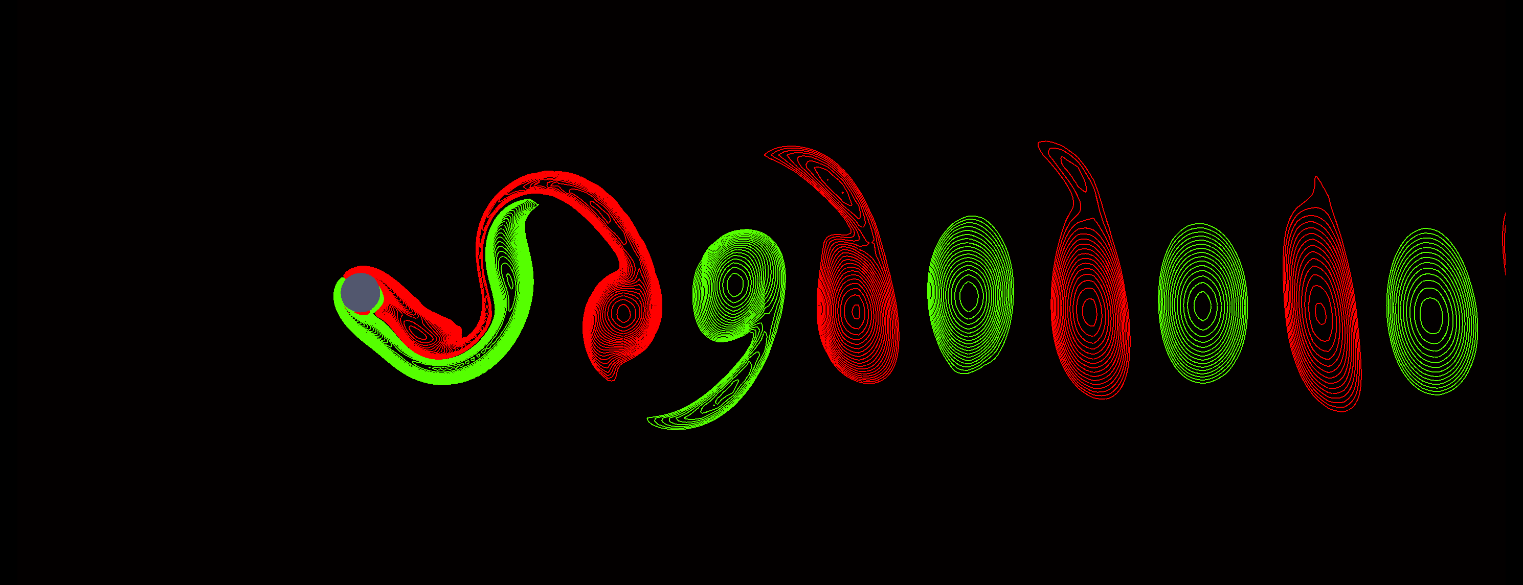
At small amplitude, it still is. The cylinder bobs gently, the 2S pattern distorts a little to follow it, and the wake keeps its top–bottom symmetry. Past a threshold amplitude, something else happens: the vortices stop alternating cleanly. Two vortices of the same sign shed close together from one side, then a single from the other. The wake reorganises into a P+S pattern — a pair and a single — repeating once per forcing period:
This is, on the face of it, surprising. The forcing is symmetric. The cylinder is round. The free stream is uniform. Every input has reflective symmetry, and yet the output breaks that symmetry: the wake either tilts up or it tilts down, and once it’s chosen, it stays.
4. The question
Why does this happen?
Two competing answers.
Continuous topological evolution. The streamlines of the wake deform smoothly as $A$ grows. What looks like a “transition” is just the eye finally noticing a feature that was always there — the asymmetry was hiding inside the 2S pattern, and the wiggle made it visible. Mathematically, the same solution branch persists; only its appearance changes.
Bifurcation of the Navier–Stokes equations. As $A$ crosses a critical value, the symmetric solution loses stability. New, asymmetric solution branches appear. The wake doesn’t smoothly deform — it hops onto a different branch entirely. Two such branches typically appear in pairs (the “tilt up” and “tilt down” cases), and the system has to pick one.
Both stories predict the same end state: an asymmetric wake at high $A$. They differ in the mechanism, and that mechanism question is exactly what the thesis was set up to answer. The picture you get for one is fundamentally different from the picture you get for the other.
5. Why direct computation matters
To resolve the question, you need solutions of the unsteady Navier–Stokes equations at every $A$ of interest, identified as branches you can follow.
The lazy approach: pick an $A$, time-step from some initial condition, wait until things “look settled,” then call whatever you’ve got the answer. Two problems with that. First, transients can run hundreds of forcing periods — the system has to forget where it started before its long-term behaviour is visible, and that’s a lot of computation per $A$. Second, time-stepping only finds stable solutions. Unstable branches matter for understanding the picture — they’re the boundaries between basins of attraction — and you can never see them by integrating forward.
The alternative is to treat the limit cycle as the unknown. Write the periodic solution as a boundary-value problem in space-time:
$$ u(x, y, t + T) = u(x, y, t) $$
— i.e. solve directly for $u$ on a domain that’s spatial in $(x, y)$ and circular in $t$, with the period $T$ either fixed (when forcing pins it) or itself an unknown (autonomous shedding). The Navier–Stokes equations are still the residual; periodicity is enforced as a constraint instead of being waited for.
That changes the problem from time-integration to root-finding. Discretise the space-time system, hand the resulting nonlinear system to Newton iteration, and you converge in a handful of steps when you converge at all. To follow a branch as $A$ varies, wrap the whole thing in arc-length continuation: even when the branch folds back on itself or passes through a bifurcation, you can keep going.
The trade-off is concrete. Bigger linear system per step, but orders of magnitude fewer steps, and access to the unstable branches that time-integration can never reach. For the kind of bifurcation tracking the thesis needed, this is the only practical option.
6. The numerical method, briefly
A short sketch, no derivations.
The discretisation is a space-time finite-element method. Spatial unknowns live on adaptive meshes — refined around the cylinder where gradients live, coarse far downstream. Time is not peeled off and stepped through separately; it joins $(x, y)$ as a third finite-element direction, and the periodic solution is computed as a single boundary-value problem with $u(x, y, t+T) = u(x, y, t)$ enforced as a periodic boundary condition.
The interesting choice is which test and trial spaces to use in the time direction. The thesis uses a Galerkin-Petrov formulation in time: trial functions are continuous piecewise polynomials, test functions are one degree lower. The asymmetry matters. It produces a discretisation matrix whose time-direction couplings “look backwards” only — each time slab depends on its predecessors but not its successors, even though the global problem is periodic. The result is block-bidiagonal in time, with one corner block closing the loop. A symmetric Galerkin choice would couple every slab to its neighbours on both sides and lose that structure.
Newton iteration solves the resulting nonlinear system. Each step is a single solve of a sparse but very large linear system, handled by preconditioned Krylov. Tracing a solution branch as $A$ varies wraps the whole procedure in arc-length continuation: $A$ becomes a free variable, an extra parametric constraint pins arc length along the branch, and the augmented system is solved together. That handles fold points, pitchforks, and isolas without special-casing.
The implementation lives in oomph-lib, the open-source finite-element library this work was built on. Years of follow-up CMake work to that codebase started here.
7. The picture that came out
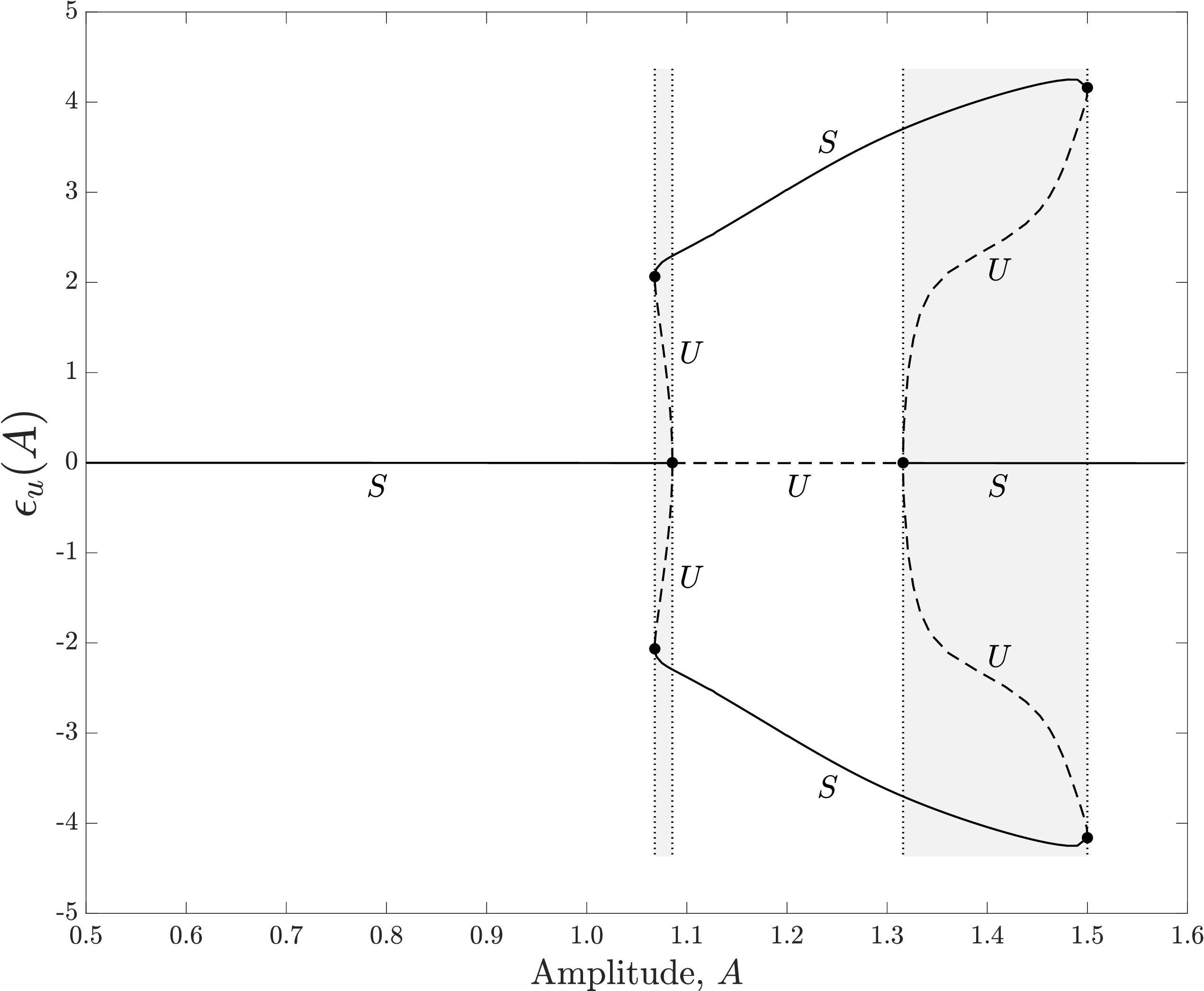
Run continuation with $A$ as the free parameter. Pick a response measure — any scalar that separates the symmetric solution from its asymmetric siblings — and plot it against $A$. The result has structure.
The ordinate is custom-built for this problem. The 2S solution has a spatio-temporal symmetry: translate by $T/2$ in time, reflect across the wake centreline, and it maps onto itself. Take the space-time finite-element solution, apply that shift-and-flip, and subtract from the original. The $L^2$ norm of the difference vanishes (to numerical precision) on the 2S branch and is non-zero on P+S. The $y$-axis plots that norm restricted to the streamwise velocity component — called $\epsilon_u$.
Below a critical amplitude $A_c$ the curve has a single branch: the 2S solution, symmetric, stable. At $A_c$ the branch forks. Two new branches grow out of it, both asymmetric and mirror images of each other — one with the pair on top and the single on the bottom, the other reflected. The symmetric branch persists past $A_c$ but loses stability there; only the asymmetric branches are physically observable past the fork. The shape is a classical pitchfork, and the geometry of its symmetry-broken solutions is what the §3 video shows at one specific point along one of those branches.
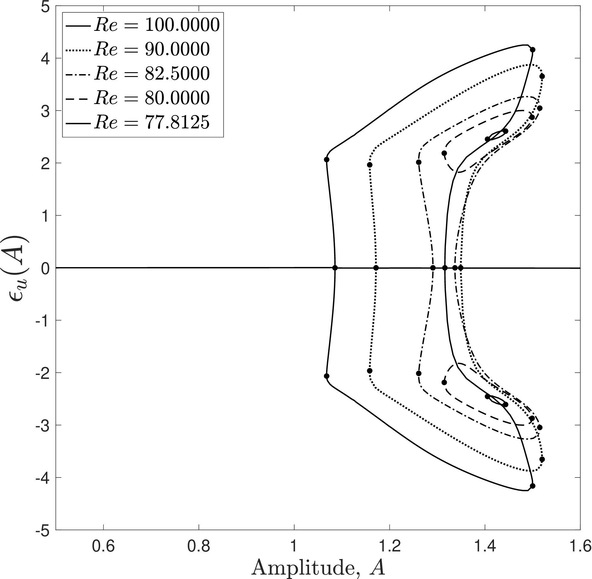
Sweeping Reynolds number alongside $A$ traces the pitchfork’s critical $A_c(\text{Re})$ across a 2D parameter plane. On one side of that curve the symmetric branch is stable; on the other, the asymmetric branches are. Continuation also finds isolas — closed loops of solution branches sitting in parameter space disconnected from the main 2S branch of solutions. Isolas are interesting because they are invisible to time-integration: starting from any natural initial condition outside the loop, the solver lands on the main branch and never visits the pocket. Continuation, on the other hand, can step onto an isola via its saddle-node birth point and traverse the closed curve.
That is the macroscopic picture: which solution lives where, and where it loses stability. Zooming in to the wake itself reveals a second layer. As $A$ approaches $A_c$, critical points of the streamline pattern — saddles, centres — slide around the wake. At $A_c$ they collide, annihilate, and reappear in a new arrangement. That local rearrangement is what the eye perceives as “the 2S wake reorganising into P+S,” and it can be characterised in its own right as a sequence of topological bifurcations of the velocity field. The two layers — solution-branch bifurcation in parameter space, topological bifurcation in the wake — are two views of the same underlying transition.
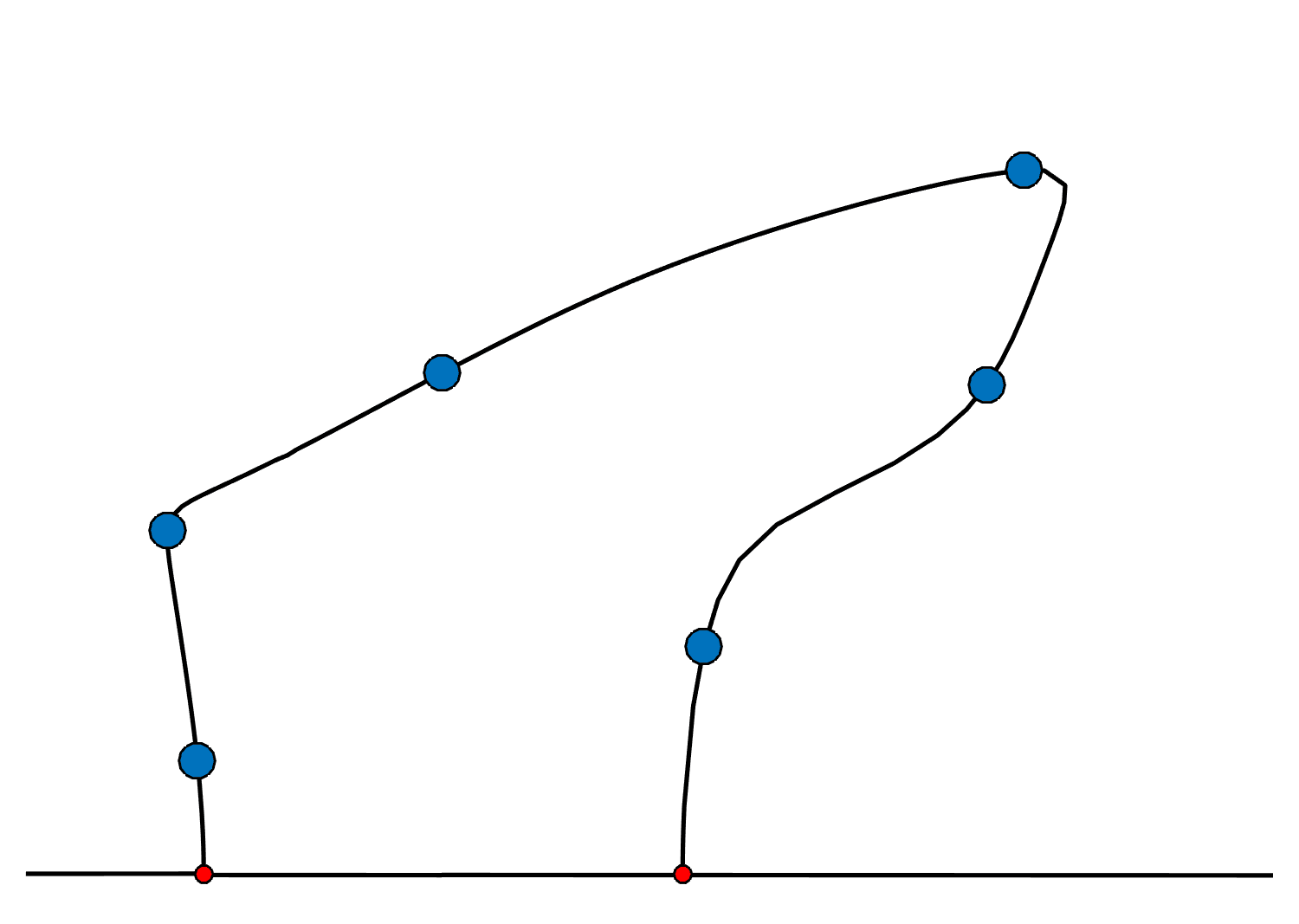
Drag the scrubber under the small bifurcation diagram below to walk the closed loop of the P+S$^{-}$ branch at six computed points. The blue ring tracks your position; the wake updates above.
8. What was novel
Two papers came out of the thesis, both in the Journal of Fluid Mechanics.
The first — Spatio-temporal symmetry breaking in the flow past an oscillating cylinder (2021) — characterises the symmetry-breaking transition itself. It shows the 2S → P+S reorganisation is a genuine bifurcation of the Navier–Stokes equations, not a continuous deformation: at the critical amplitude the symmetric solution loses stability and asymmetric branches appear. The paper traces those branches across the parameter plane.
The second — Topological bifurcations in the transition from two single vortices to a pair and a single vortex in the periodic wake behind an oscillating cylinder (2022) — drills into the topology of the streamlines as the wake moves between patterns. It identifies the critical points (saddles, centres) that appear and disappear as $A$ crosses the bifurcation, and shows how their motion organises the rearrangement.
Together they answer the §4 question: the transition is a bifurcation, and the topological evolution of streamline features is the consequence of that bifurcation, not its cause.